Introduction to Macroeconomics
22. Keynesian Macroeconomics
Contents
- John Maynard Keynes
- Short-Run Model of Aggregate Demand
- Horizontal aggregate supply (AS) function
- Aggregate Expenditures
- Consumption
- Simple Equilibrium Model
- Simplify Aggregate Expenditure Equation
- Graph the Consumption Function
- The 45o Line
- Equilibrium
- Shifts in Consumption Function
- Add Investment to the Model
- Investment
- Add Autonomous Investment to Aggregate Expenditures
- Equilibrium (assuming no government)
- Disequilibrium
- Autonomous Spending Multiplier
- Recessionary and Inflationary Gaps
- Add Government Spending to Model
- Government Spending
- Add Autonomous Government Spending
- Government Spending Multiplier
- Add Government Taxes to Model
- Lump Sum Tax
- Lump Sum Tax Multiplier
- Balanced Budget Multiplier

1. John Maynard Keynes
- Wrote General Theory of Employment, Interest, and Money (1936)
- Discounted the Classical model cornerstones of interest rate, price and wage flexibility.
Supply doesn't create its own demand, supply responds to changes in demand
- Possible to have equilibrium at less than full-employment output because of inadequate demand
- Advocated government fiscal policy activism (increase government spending and/or cut taxes) to stimulate economy

2. Short-Run Model of Aggregate Demand
- Horizontal aggregate supply (AS) function
Changes in demand lead to changes in output. For example, with a decrease in demand:
- Prices tend not to go down so you get no stimulus to consumption spending (prices and wages are downward "sticky"). The reason for price stickiness may be non-economic (people are reluctant to accept lower paying jobs even when unemployed) or economic (union wage contracts may prevent firms from cutting wages and thereby reducing prices, or firms may be reluctant to reduce wages because it reduces their workers' incentive to make a good effort).
- Interest rates have only long-run effects on consumption and investment. During a recession or depression real interest rates may be close to zero and cannot fall any further. Moreover, with a decline in demand there is no incentive for firms to increase investment spending if their factories are operating at less than full capacity.
Consequently, with a decline in demand firms have little choice but to reduce output and layoff workers. The quantity supplied responds to changes in demand.
Figure 22-1. Keynesian Aggregate Supply and Aggregate Demand

- Aggregate Expenditures
AE = C + I + G + (X - M)
- where,
- AE = Aggregate Expenditures (e.g., real GDP)
C = Consumption
I = Investment
G = Government Spending
X - M = Net exports = Exports (X) - Imports (M)

3. Consumption
Consumption Function
Consumption is assumed positive function of disposable income:
C = C0 + b * Yd
- where,
- C = total consumption expenditures
C0 = autonomous consumption (see below)
b = marginal propensity to consume (see below)
Yd = disposable income
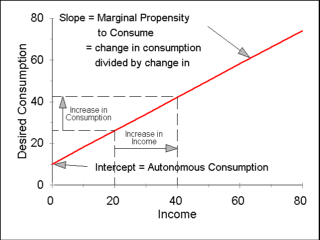
Figure 22-2. Keynesian Consumption Function

- Other non-income factors that may affect consumption (weather, wealth, interest rate, prices) assumed constant
- Since prices are assumed constant, no need for distinction between nominal and real income (important in next chapter)
- Consumption function represents "planned" or "desired " level of consumption expenditures for a given level of income
Autonomous Consumption
| Autonomous consumption |
= consumption independent of level of income |
| |
= intercept of consumption function (C0) |
Marginal Propensity to Consume (MPC)
Marginal Propensity
to Consume (MPC) |
= |
increase in consumption
per one dollar increase in disposable income |
| |
= |
change in consumption
change in disposable income |
| |
= |
dC
dYd |
| |
= |
slope of consumption function (b) |
Consumption, C = C0 + MPC * Yd
where, 0 < MPC < 1

4. Simple Equilibrium Model
To develop our model we will start small and build onto it. As we build it up we will find that the analysis really doesn't change. We will create a graph of aggregate expenditures as a function of national income. This graph is commonly referred to as the "Keynesian cross."
- Simplify Aggregate Expenditure Equation
AE = C + I + G + (X - M)
Assume no investment: I = 0
No government spending: G = 0
No international trade: X - M = 0
No corporate retained earnings, etc.: national income = personal income
No government: Personal income = disposable income
Bottom line:
AE = C
In equilibrium: total spending = total income, hence
Consumption (C) = national income (Y)
- Graph the Consumption Function
- Consumption function:
C = C0 + MPC * Y
- Aggregate expenditures:
AE = C = C0 + MPC * Y
- Graph aggregate expenditures (consumption) on vertical axis versus income on horizontal axis
Figure 22-3. Aggregate Expenditures with Consumption Only

- Autonomous Consumption
- Intercept on vertical axis (C0 in consumption function
- Consumption at $0 income (subsistence consumption)
- Consumption independent of level of income
- Dissaving: consumption is greater than income
- Marginal Propensity to Consume (MPC) = slope of consumption function
- Savings function/schedule - skip
- The 45o Line
All points of potential equilibrium, where Aggregate Expenditures = National Income
- Equilibrium
Where aggregate expenditures (consumption function) crosses the 45o line indicates the equilibrium point where desired aggregate expenditures = total income.
- Shifts in Consumption Function
Changes in factors that affect consumption other than income (e.g., a wave of pessimism that reduces the desire of people to spend money on consumption goods at any level of income)
- Cause a change in autonomous consumption (C0)
- Consumption line shifts up or down (intercept changes) but slope remains the same
- Changes the equilibrium level of aggregate expenditures and national income, i.e., supply responds to changes in demand

5. Add Investment to the Model
Add investment to create a model of what is called a closed (no exports or imports) private (no government spending or taxes) economy.
- Investment
Assumed to be autonomous (independent of level of income):
I = I0
Other non-income factors that may affect investment assumed constant until we ask "what if" under Autonomous Spending Multiplier below.
- Add Autonomous Investment to Aggregate Expenditures
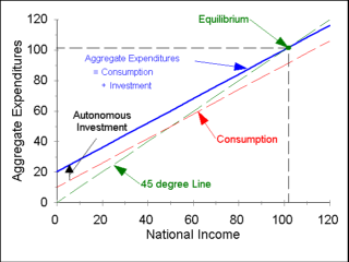
Figure 22-4. Aggregate Expenditures with Consumption and Investment

| AE |
= |
C + I |
| |
= |
C0 + MPC * Y + I0 |
- where,
- C = C0 + MPC * Y
I = I0
- Equilibrium (assuming no government)
- Graph aggregate expenditures (vertical axis) versus National Income (horizontal axis)
- Equilibrium occurs where Aggregate expenditures curve crosses the 45o line
- Savings = Investment in equilibrium (when there is no government)
Aggregate expenditures = National Income at equilibrium
AE = Y
Where, aggregate expenditures = consumption + investment
C + I = Y
Rearranging,
I = Y - C
From definition of Savings (Y = S + C, or S = Y - C),
I = S
- Disequilibrium
- National Income > Aggregate Expenditures
- Production (income) greater than spending
- on Keynesian cross, income to right of equilibrium level
- implies production, which generates income, is greater than aggregate expenditures, or quantity supplied is greater than the quantity demanded.
- undesired inventory accumulation
- economy returns to equilibrium when:
- output and income declines
- consumption declines but not as fast as income because of MPC
- hence, production declines faster than spending until equilibrium restored
- National Income < Aggregate Expenditures
- Production (income) less than spending
- on Keynesian cross, income to left of equilibrium point
- undesired inventory decline
- Economy returns to equilibrium when:
- output and income increases
- consumption increases but not as fast as income because of MPC
- hence, production increases faster than spending until equilibrium restored
- Unlike Classical model and Say's law, here output responds to a given level of demand. output does not create its own demand.

6. Autonomous Spending Multiplier
Two questions:
- What happens to total private spending and national income if there is a change in autonomous consumption or autonomous investment?
- If the economy is in a recession, how much of an increase in autonomous spending is needed to increase aggregate expenditures and national income to level of full-employment output?
| Autonomous Spending Multiplier |
= |
change in national income and output
change in autonomous investment |
| |
= |
1
1 - MPC |
- Graphical Derivation of the Autonomous Spending Multiplier

Big bang for the buck - the change in national income is much larger than the change in autonomous spending because of the multiplier effect
- Algebraic derivation of the Autonomous Spending Multiplier
AE = C + I
= C0 + MPC * Y + I0
In equilibrium:
Y = AE
Hence,
Y = C0 + MPC * Y + I0
Collect Y terms on the left:
Y - MPC * Y = C0 + I0
(1 - MPC) * Y = C0 + I0
Solve for Y:
| Y = |
1
1 - MPC |
* (C0 + I0) |

7. Recessionary and Inflationary Gaps
Characterize changes in total spending and/or income to return economy to equilibrium at full-employment output
Recessionary (Contractionary) Gap
- Equilibrium less than full-employment output
- Recessionary Gap = amount by which total expenditures fall short of total required for equilibrium and full-employment output
- Measured by vertical distance from total planned expenditure line up to the 45o line at full-employment output (national income)
Inflationary (Expansionary) Gap
- Equilibrium higher than full-employment output
- Inflationary Gap = amount by which total expenditures exceed total required for equilibrium and full-employment output
- measured by vertical distance from total planned expenditure line down to the 45o line at full-employment output (national income)
Output Gap
Output Gap (not in text)- measured along horizontal axis (national income)
Spending must increase by amount of recessionary gap or decrease by amount of inflationary gap to produce necessary change national income (output gap) to return the economy to equilibrium at full-employment output

8. Add Government Spending to Model
- Government Spending
Assumed to be autonomous (independent of level of income):
G = G0
- Add Autonomous Government Spending
| AE | = Total private spending |
| | = C + I + G |
| | = C0 + MPC * Y + I0 + G0 |
- Government Spending Multiplier
Because government spending is assumed to be autonomous, the government spending multiplier is identical to the autonomous spending multiplier:
| Change in national income and output |
= |
1
1 - MPC |
* change in autonomous government spending |

9. Add Government Taxes to Model
We will keep our model simple by considering only lump sum taxes. Lump sum taxes are independent of the level of income and this makes the analysis very similar to that for autonomous spending. If we had considered income taxes, which are a function of income, then the model would become more complicated because changes in income tax rates would not only shift the aggregate expenditure curve up and down but also change the slope of the curve.
- Lump Sum Tax
Lump Sum Tax - fixed level of total taxes (independent of level of income)
Yd = Y - T0
- where,
- Yd = Disposable income (e.g., net or take-home pay)
Y = Total income (e.g., gross pay)
T0 = Lump sum tax
Consumption shifts up or down by amount of lump sum tax, T0, times the MPC:
| Consumption |
= |
C + MPC * Yd |
| |
= |
C0 + MPC * (Y - T0) |
| |
= |
C0 + MPC * Y - MPC * T0 |
- Lump Sum Tax Multiplier
The change in national income and output arising from a $1 change in lump sum taxes is less than the change from a $1 change in autonomous government spending.
| Change in national income and output |
= - |
MPC * change in lump sum tax
1 - MPC |
Government spending multiplier larger: government spending more powerful, dollar for dollar than change in taxes. However, since President John F. Kennedy:
- tax cut less controversial
- put into effect more quickly
- more easily reversed

10. Balanced Budget Multiplier
A $1 increase in government spending matched by $1 increase in lump sum tax. Using the multipliers for changes in autonomous spending and lump sum taxes:
| Change in national income and output = |
1
1 - MPC |
* dG0 - |
MPC
1 - MPC |
* dT0 |
- where,
- dG0 = change in autonomous government spending
dT0 = change in autonomous lump sum taxes
Where change in G0 = change in T0, substitute dG0 for dT0
| Change in national income and output |
= |
1 * dG0 _ MPC * dG0
1 - MPC 1 - MPC |
| |
= |
( 1 - MPC ) * dG0,
1 - MPC 1 - MPC |
| |
= |
( 1 - MPC ) * dG0
1 - MPC |
| |
= |
change in G0 |
Bottom line: no multiplier effect. A $1 increase in government spending balanced by a $1 increase in lump sum taxes produces a $1 increase in national income.
File last modified: October 14, 2001
© Tancred Lidderdale (Tancred@Lidderdale.com)
![]()
![]()

![]()

![]()

![]()

![]()

![]()
![]()
![]()
![]()